data_vis
Introduction to data Visualization in R
 Nilanjan Chatterjee
February, 2020
Topics
- What is data visualization?
- Why is data visualization important?
- How to do data visualization?
- Possible options and pitfalls
What is data visualization?
Technique to communicate insights from data through visual representation.
Allow easy understanding of large dataset.
Provides basic knowledge about variables.
Most efficient way to identify, locate, manipulate, format, and present data.
Why data visualization is important?
- Ever increasing amount of data.
- Humanly impossible to see distinct patterns.
- Improved insight.
- Faster Decision making.
How to do data visualization?
- Plot in Base R
- ggplot2 package and associates
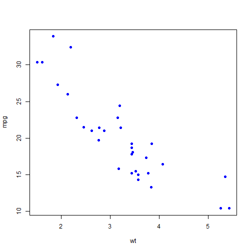
data(mtcars)
plot(mpg~wt, mtcars, pch=19, col="blue")
plot vs ggplot
plot vs ggplot
| Pros | Cons |
|---|---|
| In-built | Additional package |
| Easy to learn | Steep learning curve |
| Indepenedent of data-structures | Works only with data-frame |
| Easy for simple plots | Verbose for complex plots |
| Low level of abstraction | High abstraction level |
| Visually less appealing | Visually more appealing |
ggplot


ggplot
Based on Grammer of graphics (Wilkinson, 2005).
Consists of several building blocks like a sentence.
- data
- aesthetic mapping
- geometric object
- scales
- coordination system
- position adjustmnets
- faceting

ggplot
#install.packages("ggplot2", dependencies = T)
library(ggplot2)
ggplot(mtcars, aes(x= wt, y= mpg))+
  geom_point(colour="blue", size=3)


How to plot in ggplot
ggplot(mtcars) #data

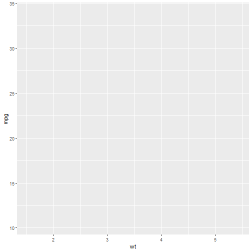
How to plot in ggplot
ggplot(mtcars, aes(x= wt, y= mpg)) #data+aesthetic map
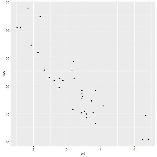
How to plot in ggplot
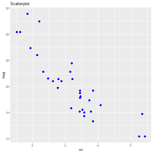
ggplot(mtcars, aes(x= wt, y= mpg))+ #data+aesthetic map
  geom_point() #geometric obj
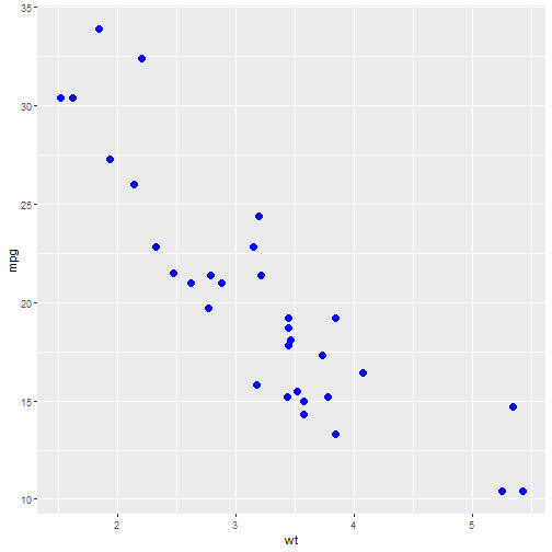
How to plot in ggplot
ggplot(mtcars, aes(x= wt, y= mpg))+ #data+aesthetic map
  geom_point(colour="blue", size=3) #geometric obj
How to plot in ggplot
ggplot(mtcars, aes(x= wt, y= mpg))+ #data+aesthetic map
  geom_point(colour="blue", size=3)+ #geometric obj
  ggtitle("Scatterplot") #Plot title
Different sections of ggplot
- DATA only data-frame is allowed
- AES takes into account the aesthetics
- GEOM stands for the different geometrices
- geom_point for point plot
- geom_bar for barplot
- geom_line for line plot
- geom_histogram for histogram
- geom_boxplot for boxplot
and so on
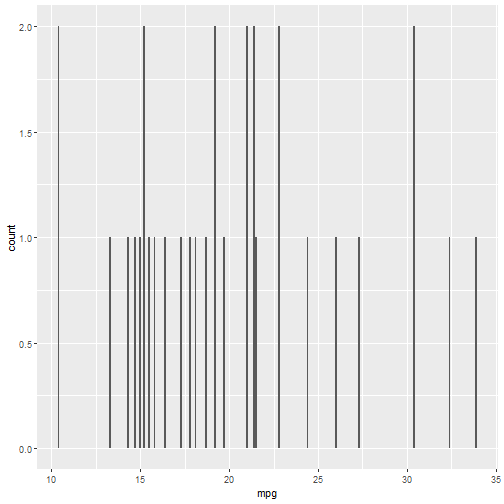
Some more examples
ggplot(mtcars, aes(x=mpg))+
  geom_bar()
Some more examples
ggplot(mtcars, aes(x=cyl, y=mpg, fill= cyl))+
  geom_bar(stat="identity")

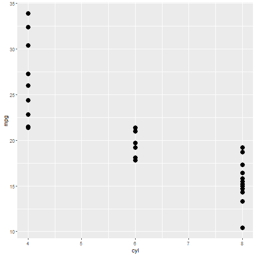
Some more examples
ggplot(mtcars, aes(x=cyl, y=mpg))+
  geom_point(stat="identity", size=4)
Export graphs from R/Rstudio
You can export any plots using the plot window from R/RStudio.
To save files in high-resolution these commands are helpful
sct <-ggplot(mtcars, aes(x= wt, y= mpg))+
  geom_point(colour="blue", size=3)+   ggtitle("Scatterplot")

ggsave(sct, "Scatterplot_with_R.jpeg", dpi=100, device = "jpeg")
Exercise
- Use your own data and make a basic plot (scatterplot, barplot, histogram) in ggplot
- change the color of the plot
- What is the difference if you put colour or shape in data part rather than geometric object part?
Thanks
- For further queries nilanjan@wii.gov.in
- Slides: https://nilanjanchatterjee.github.io/projects/
